
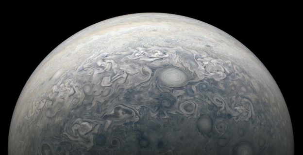
Polar view of Jupiter by Juno JUNOCAM at Perijove 72.
Credit: NASA/JPL-Caltech/SwRI/MSSS/Kevin M. Gill © CC BY
Credit: NASA/JPL-Caltech/SwRI/MSSS/Kevin M. Gill © CC BY
Description
Raw images were selected from the 4-color JunoCam database with central wavelength and FWHM as follows: 480.1nm/45.5 nm, 553.5 nm/79.3 nm, 698.9 nm/175.4 nm and 893.3 nm/22.7 nm. JunoCam flat fields were generated and mapped onto HST wavelength reflectance files for 5 HST filters: F275W, F305N, F502N, F631N and FQ889N.
This dataset contains machine learning-based processing of JunoCam images (“input images") to provide equivalent reflectance values in Hubble filter wavelengths (“generated images"). The dataset is divided into full globe mosaics of the JunoCam images in equirectangular planetographic coordinates and also into smaller tiles in the Lambert Azimuthal Equal Area (LAEA) projection.
The JunoCam data used as input to the model are generated by processing the raw images from the Mission Juno website, following the method of Sankar et al. (2024). Each individual image is processed as follows:
1. Retrieve the raw images and metadata from the Mission Juno website
2. De-compand the images using the look-up table to revert to the 12-bit data.
3. Find the jitter in the camera time by sampling a range of possible jitter values in increments of 1ms. The best jitter value is the one where the distance between the projected limb pixel positions (red line, for that jitter value) and the observed limb (green line) is minimized.
4. Apply a flat-field for each framelet
5. Determine the longitude/latitude coordinates of each pixel
6. Project the image to a cylindrical (planetographic) coordinate system centered at (0, 0) lon/lat.
7. Flatten the image by applying a high pass Gaussian filter. This works by applying a Gaussian filter on the image and the corresponding image “footprint" (i.e., a binary mask of the image where data exists). The highpass version of the image is obtained by dividing the original by the filtered image and multiplying by the footprint (to remove artifacts at the edge). The filtered footprint is then cut at the 80% value to trim the edges (where filtering artifacts occur).
8. The flattened images are stacked together to generate a global mosaic These steps generate JunoCam mosaics per perijove, which are then cropped to produce 16,000×16,000 km segments in the LAEA projection. These segments are used as input to both train the model as well as to generate the final calibrated dataset.
References
Hansen, C. J., Caplinger, M.A., Ingersoll, A., Ravine, M.A., Jensen, E., Bolton, S., Orton, G., 2017, Junocam: Juno’s Outreach Camera, Space Science Rev., doi: 10.1007/s11214-014-0079-x
Kim, B., Kwon, G., Kim, K., & Ye, J. C. 2024, in ICLR
Punnappurath, A., Abuolaim, A., Abdelhamed, A., Levinshtein, A., & Brown, M. S. 2022, in Proceedings of the IEEE/CVF Conference on Computer Vision and Pattern Recognition (CVPR)
Sankar, R., Brueshaber, S., Fortson, L., et al. 2024, Planetary Science Journal, 5, 203, doi: 10.3847/PSJ/ad6e75
Simon, A. A., Wong, M. H., & Orton, G. S. 2015, The Astrophysical Journal, 812, 55, doi: 10.1088/0004-637X/812/1/55
Zhu, J.-Y., Park, T., Isola, P., & Efros, A. A. 2017, in 2017 IEEE International Conference on Computer Vision (ICCV)
Accessing the Data
Kim, B., Kwon, G., Kim, K., & Ye, J. C. 2024, in ICLR
Punnappurath, A., Abuolaim, A., Abdelhamed, A., Levinshtein, A., & Brown, M. S. 2022, in Proceedings of the IEEE/CVF Conference on Computer Vision and Pattern Recognition (CVPR)
Sankar, R., Brueshaber, S., Fortson, L., et al. 2024, Planetary Science Journal, 5, 203, doi: 10.3847/PSJ/ad6e75
Simon, A. A., Wong, M. H., & Orton, G. S. 2015, The Astrophysical Journal, 812, 55, doi: 10.1088/0004-637X/812/1/55
Zhu, J.-Y., Park, T., Isola, P., & Efros, A. A. 2017, in 2017 IEEE International Conference on Computer Vision (ICCV)
The data has 2 components:
Data calibrated, A series of tif files of images for individual orbits
Data mosaics, A series of fits files.
Data mosaics, A series of fits files.
The User’s guide and the following indexes are available for assistance in accessing the data.
Calibrated Index (csv)
Mosaic Index (csv)
Citations
PDS recommendations for citing data sets can be found here.
G. Georgakis, R. Sankar, E.K. Dahl, B. Bucher, M. Wong, G. Eichstädt, A.P. Singh, S. Shah (2026). JunoCam - Machine Learning Calibration Bundle, NASA Planetary Data System, https://www.doi.org/10.17189/ryea-mj65.